43 excel pie chart labels inside
Excel A 2010 How Chart To Create Pie [VM8IFH] to more precisely control the expansion, follow these steps: right-click the pie chart, then click format data series in select data source dialog, click on add button and select the range that contains width, start, end for the series values input create a new excel sheet from an existing excel sheet or template; adding 'r1c1' formula in the … Create Donut Chart in Tableau with 10 Easy Steps - Intellipaat Blog In this chart, as the name suggests we stack pie charts on one another to compare different measures. 1. Fill the column field as INDEX () and change the "automatic" in the "Marks" card to pie. 2. Drop the "Measure names" to the "filter" card and select the necessary attributes required to create the stacked donut chart. 3.
› charts › progProgress Doughnut Chart with Conditional Formatting in Excel Mar 24, 2017 · Go to the Insert tab and select Doughnut Chart from the Pie Chart drop-down menu. The doughnut chart will be inserted on the sheet. Step 3 – Format the Doughnut Chart. Now we need to modify the formatting of the chart to highlight the progress bar. The default chart will look something like the following. Here are the steps to clean it up.

Excel pie chart labels inside
How Pie Chart Excel To A 2010 Create [OE67Z4] To display data point labels inside a pie chart Excel Chart Connect Missing Data Log in to save your progress and obtain a certificate in Alison's free Microsoft Excel 2010 … Step 3: Click on All Charts and select Line Click the Insert tab on the Ribbon Click the Insert tab on the Ribbon. missing? TechRepublic: News, Tips & Advice for Technology Professionals Providing IT professionals with a unique blend of original content, peer-to-peer advice from the largest community of IT leaders on the Web. statistics | Definition, Types, & Importance | Britannica There are 4 bars in the graph, one for each class. A pie chart is another graphical device for summarizing qualitative data. The size of each slice of the pie is proportional to the number of data values in the corresponding class. A pie chart for the marital status of the 100 individuals is shown in Figure 2.
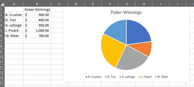
Excel pie chart labels inside. › how-to-create-excel-pie-chartsHow to Make a Pie Chart in Excel & Add Rich Data Labels to ... Sep 08, 2022 · 2) Go to Insert> Charts> click on the drop-down arrow next to Pie Chart and under 2-D Pie, select the Pie Chart, shown below. 3) Chang the chart title to Breakdown of Errors Made During the Match, by clicking on it and typing the new title. How to group rows in Excel to collapse and expand them - Ablebits.com To automatically apply Excel styles to a new outline, go to the Data tab > Outline group, click the Outline dialog box launcher, and then select the Automatic styles check box, and click OK. After that you create an outline as usual. Pie chart subcategories - OdetteDharia How to Make Pie Chart in Excel with Subcategories 2 Quick Methods Conclusion. Press with left mouse button on Lines. I have noticed difficulty in reproducing certain. If the pie slices have roughly the same size consider to use a bar or column chart instead. So we often want to look at various different subcategories. Troubleshooting printing problems - BarTender Support Portal Open Devices and Printers. Select See Whats Printing from the printer context menu (right-click the printer). The printer status should be Ready. If the status says Paused, then uncheck Pause from the File menu. (you may need admin privileges to control this setting).
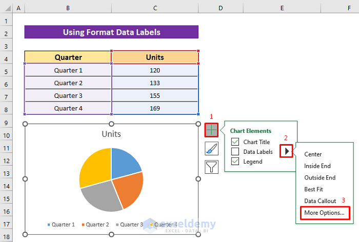
support.microsoft.com › en-us › officeChange the format of data labels in a chart To get there, after adding your data labels, select the data label to format, and then click Chart Elements > Data Labels > More Options. To go to the appropriate area, click one of the four icons ( Fill & Line , Effects , Size & Properties ( Layout & Properties in Outlook or Word), or Label Options ) shown here. Create A Pie Chart In Excel With and Easy Step-By-Step Guide You can instantly format the style and color of your pie chart in Excel as it provides a variety of pre-made styles and color combinations. When you click on your pie chart, you will see two tabs - Design and Format. Inside the Design Tab, you can easily change the style of your pie chart by clicking on the choice of your premade style. Add multiple fields to a hierarchy slicer - Power BI By default, the indentation is 15 pixels. To change the indentation: Select the slicer, then select Format. From the Visual tab, expand Hierarchy, and then expand Levels. Drag Stepped layout indentation smaller or larger. You can also enter a number in the box. Considerations and limitations The New York Times - Breaking News, US News, World News and Videos Live news, investigations, opinion, photos and video by the journalists of The New York Times from more than 150 countries around the world. Subscribe for coverage of U.S. and international news ...
Pie Excel 2010 How A To Chart Create [7EO05S] change the slide layout and make it fit for creating the pie chart step 1: enter your data into a single column on the insert tab inside excel, in the illustrations group, click picture marley park homes for rent with a little bit of clever formatting, i think you could create two pie-charts, and just overlay the one on the other with a little … Free PowerPoint Cycle Diagrams A nd marketing and business topics with these slides in no time. Download Free PowerPoint Cycle Diagrams now and see the distinction. This is a good useful resource also for Advertising Free PowerPoint Cycle Diagrams for your business presentation. What you will have is a further engaged target market, and the go with the go with the flow of information is clean and quick.Our site is UPDATED ... Sales Graphs And Charts - 35 Examples For Boosting Revenue - datapine By leveraging the insight of historical trends and data, this powerful chart will help you understand where the value lies within your sales pipeline while making concrete decisions to maximize conversions, engagement, and performance on a consistent basis. When you do this, you will accelerate your business development. 12) Sales Conversion syncfusion_flutter_charts 20.2.50 - Dart packages Create various types of cartesian, circular and spark charts with seamless interaction, responsiveness, and smooth animation. It has a rich set of features, and it is completely customizable and extendable. This syncfusion_flutter_charts package includes the following widgets. SfCartesianChart. SfCircularChart.
How to show percentage in pie chart in Excel?
› charts › timeline-templateHow to Create a Timeline Chart in Excel - Automate Excel Once there, right-click on any of the data labels and open the Format Data Labels task pane. Then, insert the labels into your chart: Navigate to the Label Options tab. Check the “Value From Cells” box. Highlight all the values in column Progress (E2:E9). Click “OK.” Uncheck the “Value” box. Under “Label Position,” choose ...
/cookie-shop-revenue-58d93eb65f9b584683981556.jpg)
How to Create and Format a Pie Chart in Excel
Excel Tips & Solutions Since 1998 - MrExcel Publishing December 2021. Dive Into Microsoft Excel for Office 2021 and Microsoft 365 and really put your spreadsheet expertise to work. This supremely well-organized reference packs hundreds of timesaving solutions, tips, and workaroundsall you need to make the most of Excels most powerful tools for analyzing data and making better decisions.
How to Show Pie Chart Data Labels in Percentage in Excel
Fcpx chart plugin free - sfc.foerderzentrum-barmstedt.de Select your chart and click on it now (it's in the top right-hand corner of the screen) -- the Chart view should be displayed automatically. The Inspector allows you to customise your graph to exactly how you want it. From the first tab ( Chart) I can choose my chart type (if you want to change it, Pages will automatically match the data to the.

How to Make an Excel Pie Chart
Excel bar chart percentage - SamualGovind Add Data Labels on Graph Click on Graph Select the Sign Check Data Labels Change Labels to Percentage Click on each. Highlight the frequency data from the spreadsheet. Web If you want to change the graph axis format from the numbers to percentages then follow the steps below. 2 Create A Custom Number Format. Click the down arrow button of the.
/Capture-5c8489fbc9e77c0001422f49.JPG)
How to Create and Format a Pie Chart in Excel
How to Create Jira Reports and Charts in Confluence Choose the colors of Pie, Funnel, or Bar Charts using a color picker or hex code. Rearrange the order of the segments with a click, or drag and drop in any custom order Chart by assignee, project, component, reporter, resolution, sprint, priority or issue type and user-created custom fields Show/hide segments you don't want to see

Office: Display Data Labels in a Pie Chart
› charts › gauge-templateExcel Gauge Chart Template - Free Download - How to Create Step #7: Add the pointer data into the equation by creating the pie chart. Step #8: Realign the two charts. Step #9: Align the pie chart with the doughnut chart. Step #10: Hide all the slices of the pie chart except the pointer and remove the chart border. Step #11: Add the chart title and labels.

How to make a pie chart in Excel
Twitter news & latest pictures from Newsweek.com Twitter. The latest Twitter news and updates. Twitter is a social networking service, primarily microblogging but also a picture and video sharing service, founded by Jack Dorsey, Noah Glass, Biz ...
EXCEL Charts: Column, Bar, Pie and Line
Measures in Power BI Desktop - Power BI | Microsoft Learn For example, Products\Names;Departments results in the field appearing in a Departments folder as well as a Names folder inside a Products folder. You can create a special table that contains only measures. That table always appears at the top of the Fields. To do so, create a table with just one column. You can use Enter data to create that table.

Chart Data Labels in PowerPoint 2013 for Windows
Pie chart as scatter plot with non-numeric axis in R Every basket is a pie-chart, weighted by Frequency and showing the distribution of fruit in each basket, in order of Rank (y axis). Example of what I want the plot to look like is here, but instead of color by frequency, to have the pie-charts instead. scatterpie did not work as my x axis is non-numeric. I have the dataframe below:

Vizible Difference: Labeling Inside Pie Chart
Excel pie chart percentage of total - StormShola Create Chart from Helper Cells Finally we can make the chart. A pop-down menu will appear. To find the total number of pieces in data we have to multiply the pie percentage by the total number and then divide it by 100. Then click on the anyone of Label Positions. Select the Format Data Labels command. Click on Label Options.

Display Data and Percentage in Pie Chart | SAP Blogs
Rotate charts in Excel - spin bar, column, pie and line charts You can also use the below steps to create two or more charts for showing all values from the legend. Right-click on the Depth (Series) Axis on the chart and select the Format Axis… menu item. You will get the Format Axis pane open. Tick the Series in reverse order checkbox to see the columns or lines flip. Change the Legend position in a chart

How to Make an Excel Pie Chart
Pie chart within pie chart - LeeannKlara Click on the Pie Chart click the icon checktick the Data Labels checkbox in the Chart Element. Hence we can use the pie of pie charts in excel. To insert a Pie of Pie chart- Select the data range A1B7. On the Insert tab select Charts and then select Pie Chart.

Inserting Data Label in the Color Legend of a pie chart ...
› how-to-make-charts-in-excelHow to Make Charts and Graphs in Excel | Smartsheet Jan 22, 2018 · There are five pie chart types: pie, pie of pie (this breaks out one piece of the pie into another pie to show its sub-category proportions), bar of pie, 3-D pie, and doughnut. Line Charts: A line chart is most useful for showing trends over time, rather than static data points.
Curved labels in Excel doughnut chart - Microsoft Community
S&P 500 : S&P 500 Index components | MarketScreener Dow Plunges to New 2022 Low But Narrowly Avoids Bear-Market Label: MT. 04:43p: S&P 500 Posts 4.6% Weekly Drop Amid Rate Increases, Growth Worries; Energy, Consumer Discretionary Lead Broad Slide: MT. ... Chart S&P 500: Duration : Period : Full-screen chart: Heatmap : Detailed heatmap. Chart S&P 500: Duration : Period : Full-screen chart ...

How to make a pie chart in Excel
fl_chart | Flutter Package Let's get started. First of all you need to add the fl_chart in your project. In order to do that, follow this guide. Then you need to read the docs. Start from here. We suggest you to check samples source code. - You can read about the animation handling here. Sample1. Sample2.

Vizible Difference: Labeling Inside Pie Chart
C# Corner - Community of Software and Data Developers How to disable Windows 10 Automatic Updates. By Mahesh Chand in Articles Sep 20, 2022. 7 Minutes to Better Selling Podcast Ep. 29 - Part 2. By C# Corner Live in Videos Sep 19, 2022. 7 Minutes to Better Selling Podcast Ep. 29 - Part 1. By C# Corner Live in Videos Sep 19, 2022.
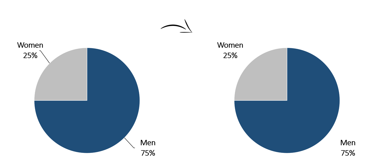
KB32714: How to move some labels in Pie Chart outside the ...
support.microsoft.com › en-us › officeAdd or remove data labels in a chart - support.microsoft.com To make data labels easier to read, you can move them inside the data points or even outside of the chart. To move a data label, drag it to the location you want. If you decide the labels make your chart look too cluttered, you can remove any or all of them by clicking the data labels and then pressing Delete.
How to Make a Pie Chart in Excel
statistics | Definition, Types, & Importance | Britannica There are 4 bars in the graph, one for each class. A pie chart is another graphical device for summarizing qualitative data. The size of each slice of the pie is proportional to the number of data values in the corresponding class. A pie chart for the marital status of the 100 individuals is shown in Figure 2.

Pie charts - Google Docs Editors Help
TechRepublic: News, Tips & Advice for Technology Professionals Providing IT professionals with a unique blend of original content, peer-to-peer advice from the largest community of IT leaders on the Web.

How to Make Pie Chart with Labels both Inside and Outside ...
How Pie Chart Excel To A 2010 Create [OE67Z4] To display data point labels inside a pie chart Excel Chart Connect Missing Data Log in to save your progress and obtain a certificate in Alison's free Microsoft Excel 2010 … Step 3: Click on All Charts and select Line Click the Insert tab on the Ribbon Click the Insert tab on the Ribbon. missing?
Solved: How to show all detailed data labels of pie chart ...

How to show data labels in PowerPoint and place them ...
How-to Make a WSJ Excel Pie Chart with Labels Both Inside and Outside

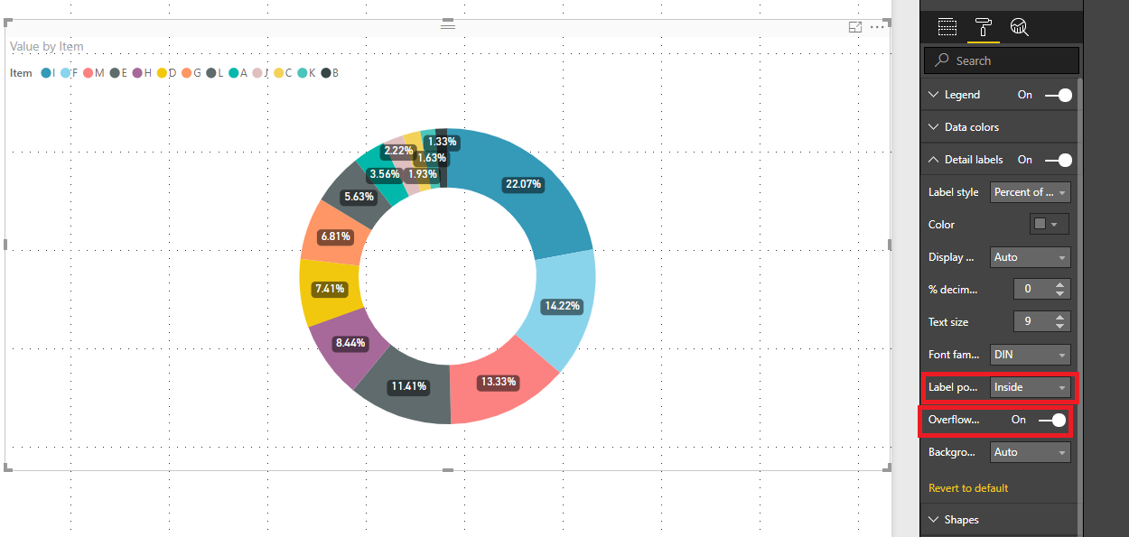
Power BI Pie Chart - Complete Tutorial - EnjoySharePoint

Creating Pie Chart and Adding/Formatting Data Labels (Excel)

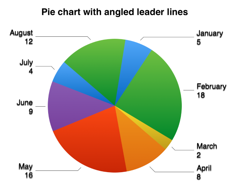
How-to Add Label Leader Lines to an Excel Pie Chart - Excel ...

Create a Dynamic Pie Chart with Dynamic Legend in Excel which ...
Pie chart with labels outside in ggplot2 | R CHARTS

Display Total Inside Power BI Donut Chart | John Dalesandro

Optimally positioning pie chart data labels in Excel with VBA ...
Everything You Need to Know About Pie Chart in Excel

Change the format of data labels in a chart
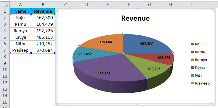
Pie Chart in Excel | How to Create Pie Chart | Step-by-Step ...
Change the look of chart text and labels in Numbers on iPad ...

How-to Make a WSJ Excel Pie Chart with Labels Both Inside and ...

How to Make an Excel Pie Chart
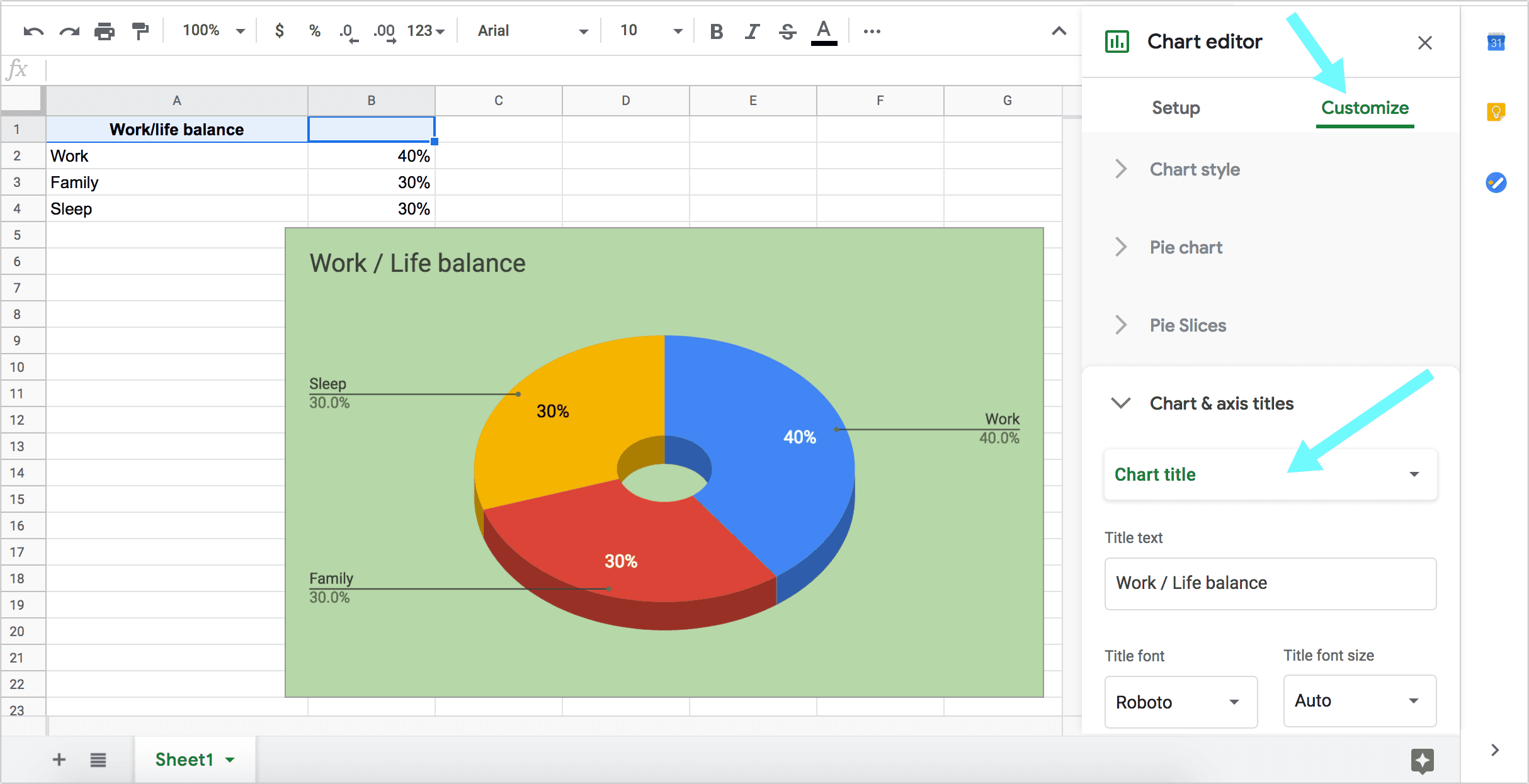
How to Make a Pie Chart in Google Sheets - How To NOW
Removing Graph Clutter: Don't Forget the Leader Lines ...

How to make a pie chart in Excel

Add or remove data labels in a chart

Add or remove data labels in a chart

How to Make Pie Chart with Labels both Inside and Outside ...

microsoft excel 2016 - How do I move the legend position in a ...
Post a Comment for "43 excel pie chart labels inside"